
Updating our ADMET Toolkits
Teaching Axon to do ADMET modeling the right way

A few weeks ago, we published a blog showing how Axon could train and evaluate molecular property prediction models for ADMET endpoints. The post walked through the full workflow—featurizing molecules, training Chemprop and classical ML models, and comparing their performance on standard public benchmarks (TDC and MoleculeNet datasets).
We received a response from Pat Walters—author of Practical Cheminformatics and Chief Scientist at OpenADMET—pointing out that the datasets and evaluation methodology we used had well-documented problems. We want Axon to promote scientific best practices, not just execute scientific methods, so we made it better.
This post describes how we updated Axon to follow Pat Walters’ wisdom with a few demonstrative examples. We hope this update enables the community to perform better molecular property prediction, and serves as a roadmap for how Axon can continually improve with user feedback.
What our toy examples missed
The dataset problem
MoleculeNet and TDC are large public benchmark collections widely used in ML papers; however, some of their datasets have problems. These problems include unparseable SMILES, undefined stereocenters, and duplicate datapoints with contradictory labels, as discussed in Walters’ blog. MoleculeNet also uses data from a variety of sources—different labs, different experimental protocols, different assay conditions—which means that the dataset is not as clean as it could be and can introduce significant noise into models trained on it, as discussed by Landrum & Riniker in the context of IC50 values from ChEMBL. Our earlier post used MoleculeNet’s blood-brain barrier (BBB) permeability and TDC’s bioavailability datasets. The BBB dataset is known to contain several of the issues mentioned above, such as unparseable SMILES and contradictory duplicate structures.
The evaluation problem
When evaluating the models Axon made, we used default Murcko scaffold splits, which are a limited heuristic for ensuring out-of-domain chemistry in a test-set. We trained five independent models and reported mean AUROC metrics, but didn’t include statistical tests for significance. Likewise, we failed to include simple baselines (e.g., a logistic regression model based on the Clark log BB equation) to contextualize the performance of the ML models.
What Axon learned
We used this opportunity to improve Axon’s world knowledge and toolkit. We compiled posts from the OpenADMET website and Walters’ personal blog, and then asked Axon how it might do things differently. It suggested several improvements and noted the priority of each, most of which we’ve since incorporated.
Curated datasets and pipelines
Polaris (
polaris-lib): Access to benchmark datasets with single-lab provenance, curated structures, and defined experimental protocols. Specifically, it contains the Biogen ADME Fang dataset—generated in one lab under consistent conditions.OpenADMET models (
openadmet-models): A modeling framework that contains deep learning, classical ML, and workflow tools for molecular property prediction with a focus on ADMET.
Trustworthy data splitting and evaluation
astartes: Principled dataset splitting—Butina clustering, scaffold-based, and temporal splits that prevent data leakage between train and test sets.mlxtend: Additional tools for machine learning evaluation and visualization that extendscikit-learnfunctionality, including the 5×2 cross-validation paired t-test for statistically valid model comparison.scikit-posthocs: Post hoc statistical tests, like the Friedman test with post-hoc corrections and Critical Difference Diagrams for comparing multiple models.
Expert interpretation
useful_rdkit_utils: Pat Walters’ own utility library—REOS structural alert filters, fingerprint tools, and functions for calculating the maximum possible correlation given experimental noise.
These tools are now available to Axon, so any user can access them in their own modeling workflows (with the exception of CReM, which proved slightly challenging and is a work-in-progress as of writing).
Beyond tools, we’ve also updated Axon’s knowledge base to include best practices outlined in Practical Cheminformatics and the OpenADMET blog. This information adjusts Axon’s behavior, guiding it to perform exploratory data analysis to check for structural alerts and contradictory datapoints, split datasets using clustering methods like Butina clustering, use appropriate statistical tests, compare ML models against simple baselines, report more than one metric to evaluate model performance.
Best practices in action
Let’s explore the impact of these updates through two illustrative questions:
Do ML models beat simple equations on realistic data?
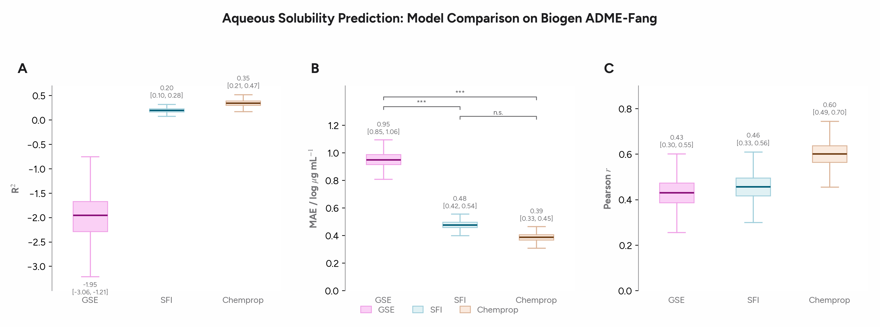
We started by asking Axon to use the Polaris Biogen solubility data from the polaris-lib package to compare several models for solubility prediction. We assessed the General Solubility Equation (GSE, which has 2 parameters: logP and melting point)1, the Solubility Forecast Index (SFI, which has 2 parameters: clogD and aromatic ring count), and a Chemprop GNN. Axon used Butina cluster splits and bootstrap confidence intervals in its comparison.
On a realistic pharma dataset with a narrower dynamic range, the gap between the 2-parameter SFI equation and the GNN is smaller than you might expect, though both outperform the GSE. The GNN wins, but modestly and not significantly. This example illustrates the importance of engaging baselines appropriate statistical tests to assess whether ML models are adding value, particularly since they are less interpretable than traditional QSAR models.
How much do splits matter?
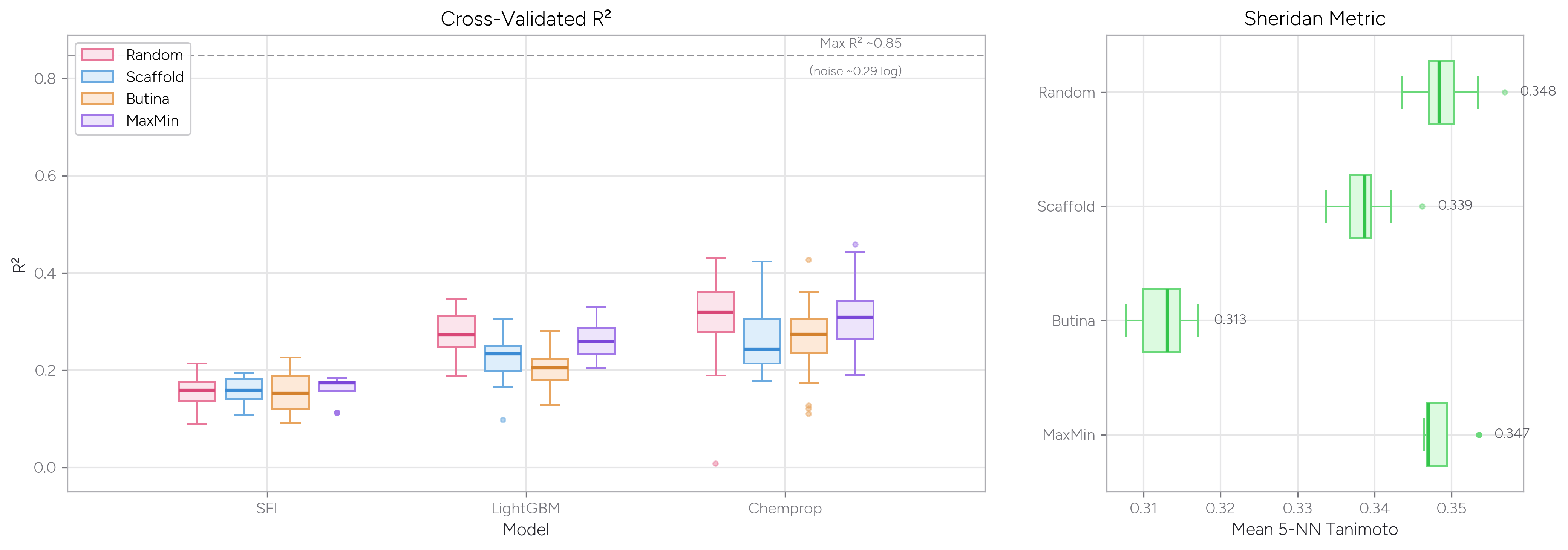
Data splits can significantly affect a model’s performance metrics. Random splits rarely reflect the reality of how molecular property data are gathered and used in practice. While the most realistic way to split a dataset is time-based splitting, which mimics how data might be collected and used in a pharmaceutical company, it’s not always possible to do so with the available data. Absent time-stamped data, scaffold-based and Butina cluster splitting can offer improvements over random splits. In scaffold splitting, molecules are grouped by their Murcko scaffolds (the core ring systems and linkers, with side chains stripped away), while in Butina clustering, molecules are grouped by their overall fingerprint (a descriptor for chemical features) similarity to one another.
Butina cluster splitting is generally considered the most rigorous option for evaluating how a model will perform on new chemistry, because it prevents structurally similar molecules from appearing in both the training and test sets. In contrast, random splits promote overlap in the training and test set distributions. “MaxMin” splitting explicitly selects for a maximally diverse training set (based on fingerprints), such that the test set is effectively testing for a model’s interpolation ability.
We asked Axon to train LightGBM and Chemprop models on solubility data and compare how these models performed when trained using random (i.e., uniformly random) splits, MaxMin splits (using the Kennard-Stone algorithm in astartes), scaffold splits, and Butina cluster splits. We also asked Axon to calculate the average Tanimoto similarity from Morgan fingerprints for each molecule in the test set to its five nearest neighbors in the training set (the Sheridan metric).
As you might expect, random and MaxMin splits give higher R2 values than the scaffold or Butina cluster splitting methods. This result makes sense: The MaxMin algorithm selects a maximally diverse test set, but those diverse test points still tend to have close neighbors in the large training set—so the model isn’t truly challenged by unfamiliar chemistry. Butina cluster splitting, by contrast, assigns whole clusters of similar molecules to one side of the split, ensuring the model must generalize to genuinely new structural territory.
Both the Sheridan metric (a measure of train vs. test set similarity) and model R2 values reflect this dynamic: when test molecules are less similar to their nearest training neighbors, model performance drops. Note also the dashed line at R2 ~0.85, which represents the maximum achievable performance given the experimental noise in this assay from useful_rdkit_utils—even a perfect model can’t exceed this ceiling.
Building Axon to be the best collaborator it can be
Our goal with this update is to show how we’re working to make Axon the best collaborator it can be for scientists. We demonstrated simple examples of the tools and datasets we’ve added—in particular for better data splitting and validation methods. These matter for any machine learning work, which is quickly becoming a staple of modern drug discovery. We are keen on incorporating feedback from users and the computational chemistry, cheminformatics, and bioinformatics communities to ensure Axon works for them.
Axon now supports these best practices out of the box. Any user can run these same analyses on their own data. We plan to continue making updates as the field evolves—particularly as OpenADMET continues publishing blind challenge results and certified datasets. We’re grateful to Pat Walters for motivating this work and for helpful discussions, as well as the OpenADMET organization for its contributions to the field.
We are excited to hear what scientists need to improve their simulation, data analysis, and visualization workflows in Axon. If you’re interested in giving it a try, you can request a demo here. If you have questions or comments or just want to talk with us, shoot me a message at alex@mirrorphysics.com.
This example is actually quite interesting beyond mere ADMET predictions: the dataset does not contain readily available melting point data needed for the GSE. Axon constructed an ad hoc equation to predict melting point based on RDKit descriptors that worked relatively well. I caught the “error” later and asked it to justify its choice, and played around with other physics-based methods like the Joback-Reid group additivity model and a more recent descriptors-based method. The GSE that used Axon’s melting point prediction method that it seemed to create on the fly performed better than the two published methods for predicting the Biogen solubility endpoint (albeit still with a negative R2 value). You can also see me tweak the figure style in the transcript above.